PivotPy
A Python Processing Tool for Vasp Input/Output. A CLI is available in Powershell, see Vasp2Visual.
Install
pip install pivotpy
How to use
Use commnad
pivotpyin regular terminal to quickly launch documentation any time.See Full Documentation.
For CLI, use Vasp2Visual.
Changelog for version 0.9.5 onward
pivotpy.s_plots.splot_rgb_linesandpivotpy.s_plots.splot_rgb_linesare refactored and no more depnd oncreate_rgb_lines, so this function is dropped, If you still want to use it, use versions below 0.9.5.A class
pivotpy.g_utils.Vasprunis added which provides shortcut forexport_vasprunand plotting functions. Under this class or as aliases:splot_bands–>sbandssplot_rgb_lines–>srgbiplot_rgb_lines–>irgbsplot_color_lines–>scolorsplot_dos_lines–>sdosiplot_dos_lines–>idosThe plot functions starting with ‘quick’ or ‘plotly’ are still working but deprecated in favor of consistent names above starting from version 1.0.3.
A class
pivotpy.g_utils.LOCPOT_CHGis added which can be used to parse and visualize files like LOCPOT and CHG.A function
pivotpy.vr_parser.split_vasprunis added which splitsvasprun.xmlfile into a small file_vasprun.xmlwithout projected data and creates text files_set[1,2,3,4].txtbased on how many spin sets are there.A function
pivotpy.vr_parser.islice2arrayis added which can reads data from text/csv/tsv files (even if text and numbers are mixed) accoridng to slices you provide, this does not load full file in memory and it is also useful in parsing EIGENVAL, PROCAR like files with a few lines of code only.Version 1.0.0 is updated with an overhaul of widgets module.
VasprunAppis introduced as class to access internals of app easily.
New: Plot in Terminal without GUI
Use pp.plt2text(colorful=True/False) after matplotlib’s code and your figure will appear in terminal. You need to zoom out alot to get a good view like below.
Tip: Use file matplotlib2terminal.py on github independent of this package to plot in terminal.
New: Ipywidgets-based GUI
See GIF here:
import os
os.chdir('E:/Research/graphene_example/ISPIN_1/bands')
xml_data=pp.read_asxml()
vr=pp.export_vasprun(elim=[-5,5])
vr
Data(
    sys_info = Data(
        SYSTEM = C2
        NION = 2
        NELECT = 8
        TypeION = 1
        ElemName = ['C']
        ElemIndex = [0, 2]
        E_Fermi = -3.35005822
        ISPIN = 1
        fields = ['s', 'py', 'pz', 'px', 'dxy', 'dyz', 'dz2', 'dxz', 'x2-y2']
        incar = Data(
            SYSTEM = C2
            PREC = high
            ALGO = N
            LSORBIT = T
            NELMIN = 7
            ISMEAR = 0
            SIGMA = 0.10000000
            LORBIT = 11
            KPOINT_BSE = -1     0     0     0
            GGA = PS
        )
    )
    dim_info = Data(
        kpoints = (NKPTS,3)
        kpath = (NKPTS,1)
        bands = ⇅(NKPTS,NBANDS)
        dos = ⇅(grid_size,3)
        pro_dos = ⇅(NION,grid_size,en+pro_fields)
        pro_bands = ⇅(NION,NKPTS,NBANDS,pro_fields)
    )
    kpoints = <ndarray:shape=(90, 3)>
    kpath = <list:len=90>
    bands = Data(
        E_Fermi = -3.35005822
        ISPIN = 1
        NBANDS = 10
        evals = <ndarray:shape=(90, 10)>
        indices = range(4, 14)
    )
    tdos = Data(
        E_Fermi = -3.35005822
        ISPIN = 1
        grid_range = range(124, 203)
        tdos = <ndarray:shape=(79, 3)>
    )
    pro_bands = Data(
        labels = ['s', 'py', 'pz', 'px', 'dxy', 'dyz', 'dz2', 'dxz', 'x2-y2']
        pros = <ndarray:shape=(2, 90, 10, 9)>
    )
    pro_dos = Data(
        labels = ['energy', 's', 'py', 'pz', 'px', 'dxy', 'dyz', 'dz2', 'dxz', 'x2-y2']
        pros = <ndarray:shape=(2, 79, 10)>
    )
    poscar = Data(
        SYSTEM = C2
        volume = 105.49324928
        basis = <ndarray:shape=(3, 3)>
        rec_basis = <ndarray:shape=(3, 3)>
        positions = <ndarray:shape=(2, 3)>
        labels = ['C 1', 'C 2']
        unique = Data(
            C = range(0, 2)
        )
    )
)
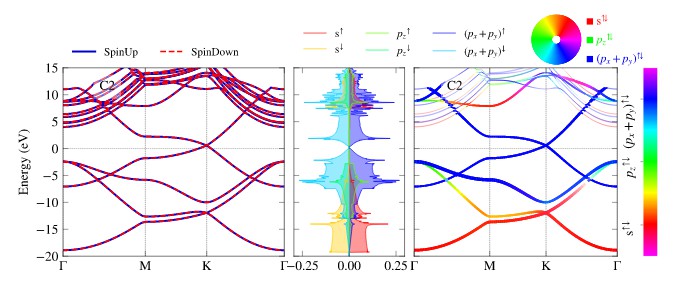
Matplotlib’s static plots
Add anything from legend,colorbar, colorwheel. In below figure, all three are shown.
Use aliases such as sbands, sdos,srgb,irgb,scolor,idos for plotting.
#collapse_input
import pivotpy as pp, numpy as np
import matplotlib.pyplot as plt
vr1=pp.export_vasprun('E:/Research/graphene_example/ISPIN_2/bands/vasprun.xml')
vr2=pp.export_vasprun('E:/Research/graphene_example/ISPIN_2/dos/vasprun.xml')
axs=pp.init_figure(ncols=3,widths=[2,1,2.2],sharey=True,wspace=0.05,figsize=(8,2.6))
elements=[0,[0],[0,1]]
orbs=[[0],[1],[2,3]]
labels=['s','$p_z$','$(p_x+p_y)$']
ti_cks=dict(ktick_inds=[0,30,60,-1],ktick_vals=['Γ','M','K','Γ'])
args_dict=dict(elements=elements,orbs=orbs,labels=labels,elim=[-20,15])
pp.splot_bands(path_evr=vr1,ax=axs[0],**ti_cks,elim=[-20,15])
pp.splot_rgb_lines(path_evr=vr1,ax=axs[2],**args_dict,**ti_cks,colorbar=True,)
pp.splot_dos_lines(path_evr=vr2,ax=axs[1],vertical=True,spin='both',include_dos='pdos',**args_dict,legend_kwargs={'ncol': 3},colormap='RGB_m')
pp.color_wheel(axs[2],xy=(0.7,1.15),scale=0.2,labels=[l+'$^{⇅}$' for l in labels])
pp._show()
[0;92m elements[0] = 0 is converted to range(0, 2) which picks all ions of 'C'.To just pick one ion at this index, wrap it in brackets [].[00m
E:\Research\pivotpy\pivotpy\s_plots.py:428: MatplotlibDeprecationWarning:
shading='flat' when X and Y have the same dimensions as C is deprecated since 3.3. Either specify the corners of the quadrilaterals with X and Y, or pass shading='auto', 'nearest' or 'gouraud', or set rcParams['pcolor.shading']. This will become an error two minor releases later.

Interactive plots using plotly
args_dict['labels'] = ['s','p_z','p_x+p_y']
fig1 = pp.iplot_rgb_lines(vr1,**args_dict)
#pp.iplot2html(fig1) #Do inside Google Colab, fig1 inside Jupyter
from IPython.display import Markdown
Markdown("[See Interactive Plot](https://massgh.github.io/InteractiveHTMLs/iGraphene.html)")
See Interactive Plot
Brillouin Zone (BZ) Processing
Look in
pivotpy.siomodule for details on generating mesh and path of KPOINTS as well as using Materials Projects’ API to get POSCAR right in the working folder with commandget_poscar. Below is a screenshot of interactive BZ plot. You candouble clickon blue points and hitCtrl + Cto copy the high symmetry points relative to reciprocal lattice basis vectors. (You will be able to draw kpath inPivotpy-Dashapplication and generate KPOINTS automatically from a web interface later on!).Same color points lie on a sphere, with radius decreasing as red to blue and gamma point in gold color. These color help distinguishing points but the points not always be equivalent, for example in FCC, there are two points on mid of edges connecting square-hexagon and hexagon-hexagon at equal distance from center but not the same points.
Any colored point’s hover text is in gold background.
Look the output of pivotpy.sio.splot_bz.
import pivotpy as pp
pp.splot_bz([[1,0,0],[0,1,0],[0,0,1]],color=(1,1,1,0.2),light_from=(0.5,0,2),colormap='RGB').set_axis_off()
#pp.iplot2html(fig2) #Do inside Google Colab, fig1 inside Jupyter
from IPython.display import Markdown
Markdown("[See Interactive BZ Plot](https://massgh.github.io/InteractiveHTMLs/BZ.html)")
See Interactive BZ Plot

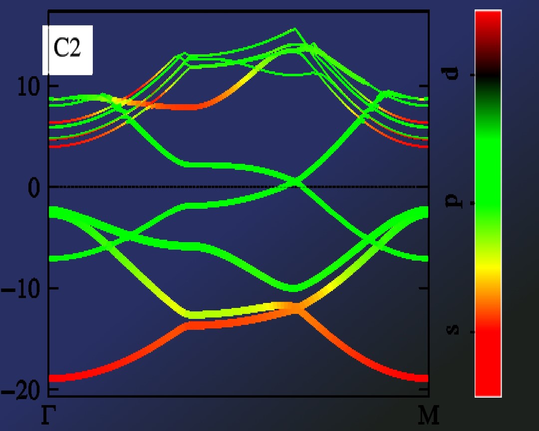
Plotting Two Calculations Side by Side
- Here we will use
shift_kpathto demonstrate plot of two calculations on same axes side by side
#nbdev_collapse_input
import matplotlib.pyplot as plt
import pivotpy as pp
plt.style.use('bmh')
vr1=pp.export_vasprun('E:/Research/graphene_example/ISPIN_1/bands/vasprun.xml')
shift_kpath=vr1.kpath[-1] # Add last point from first export in second one.
vr2=pp.export_vasprun('E:/Research/graphene_example/ISPIN_2/bands/vasprun.xml',shift_kpath=shift_kpath,try_pwsh=False)
last_k=vr2.kpath[-1]
axs=pp.init_figure(figsize=(5,2.6))
K_all=[*vr1.kpath,*vr2.kpath] # Merge kpath for ticks
kticks=[K_all[i] for i in [0,30,60,90,120,150,-1]]
ti_cks=dict(xticks=kticks,xt_labels=['Γ','M','K','Γ','M','K','Γ'])
pp.splot_bands(path_evr=vr1,ax=axs)
pp.splot_bands(path_evr=vr2,ax=axs,txt='Graphene(Left: ISPIN=1, Right: ISPIN=2)',ctxt='m')
pp.modify_axes(ax=axs,xlim=[0,last_k],ylim=[-10,10],**ti_cks)

Interpolation
Amost every bandstructure and DOS plot function has an argument interp_nk which is a dictionary with keys n (Number of additional points between adjacent points) and k (order of interpolation 0-3). n > k must hold.
#collapse_input
import pivotpy as pp
plt.style.use('ggplot')
k=vr1.kpath
ef=vr1.bands.E_Fermi
evals=vr1.bands.evals-ef
#Let's interpolate our graph to see effect. It is useful for colored graphs.
knew,enew=pp.interpolate_data(x=k,y=evals,n=10,k=3)
plot=plt.plot(k,evals,'m',lw=5,label='real data')
plot=plt.plot(k,evals,'w',lw=1,label='interpolated',ls='dashed')
pp.add_text(ax=plt.gca(),txts='Graphene')

LOCPOT,CHG Visualization
check out the class pivotpy.LOCPOT_CHG to visulize local potential/charge and magnetization in a given direction.
Running powershell commands from python.
Some tasks are very tideious in python while just a click way in powershell. See below, and try to list processes in python yourself to see the difference!
pp.ps2std(ps_command='(Get-Process)[0..4]')
NPM(K)    PM(M)      WS(M)     CPU(s)      Id  SI ProcessName
------    -----      -----     ------      --  -- -----------
15     3.32       3.91       4.86   15456   1 AdobeARM
30    20.27      68.09       4.17   14440   1 ApplicationFrameHost
8     1.56       6.52       0.00   12816   0 AppVShNotify
8     1.82       7.19       0.03   17916   1 AppVShNotify
8     1.57       5.84       0.00    5304   0 armsvc
Advancaed: Poweshell Cell/Line Magic %%ps/%ps
You can create a IPython cell magic to run powershell commands directly in IPython Shell/Notebook (Powershell core installation required).
Cell magic can be assigned to a variable
fooby%%ps --out fooLine magic can be assigned to a variable by
foo = %ps powershell_command
Put below code in ipython profile’s startup file (create one) "~/.ipython/profile_default/startup/powershell_magic.py"
from IPython.core.magic import register_line_cell_magic
from IPython import get_ipython
@register_line_cell_magic
def ps(line, cell=None):
    if cell:
        return get_ipython().run_cell_magic('powershell',line,cell)
    else:
        get_ipython().run_cell_magic('powershell','--out posh_output',line)
        return posh_output.splitlines()
Additionally you need to add following lines in "~/.ipython/profile_default/ipython_config.py" file to make above magic work.
from traitlets.config.application import get_config
c = get_config()
c.ScriptMagics.script_magics = ['powershell']
c.ScriptMagics.script_paths = {
    'powershell' : 'powershell.exe -noprofile -command -',
    'pwsh': 'pwsh.exe -noprofile -command -'
}
%%ps
Get-ChildItem 'E:\Research\graphene_example\'
    Directory: E:\Research\graphene_example


Mode                 LastWriteTime         Length Name

----                 -------------         ------ ----

da----        10/31/2020   1:30 PM                ISPIN_1

da----          5/9/2020   1:05 PM                ISPIN_2

-a----          5/9/2020   1:01 PM          75331 OUTCAR

-a----          5/9/2020   1:01 PM         240755 vasprun.xml
x = %ps (Get-ChildItem 'E:\Research\graphene_example\').Name
x
['ISPIN_1', 'ISPIN_2', 'OUTCAR', 'vasprun.xml']
GitHub
https://github.com/massgh/pivotpy
Source: https://pythonawesome.com/a-python-processing-tool-for-vasp-input-output/